Excel is a powerful tool that allows you to perform various calculations and manipulate data in a worksheet. One common issue that users often face is dealing with parentheses in their data. Whether it’s a formula or a value in a cell, parentheses can sometimes interfere with the desired calculations or formatting.
Fortunately, Excel provides several functions and techniques to remove parentheses from your data. By using these methods, you can easily extract the content within the parentheses or remove them altogether, depending on your needs.
One way to remove parentheses in Excel is by using the REPLACE function. This function allows you to replace specific characters or text within a cell with new content. By specifying the opening and closing parentheses as the characters to be replaced, you can effectively remove them from your data.
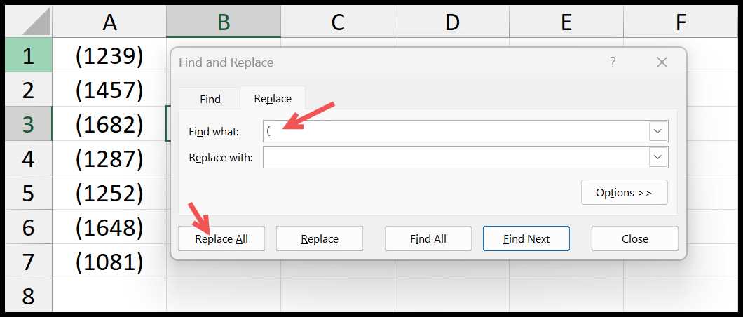
Another method to remove parentheses is by using the Find and Replace feature in Excel. This feature allows you to search for specific characters or text within a worksheet and replace them with new content. By entering the opening and closing parentheses in the “Find” field and leaving the “Replace” field blank, you can effectively remove the parentheses from your data.
Whether you’re dealing with formulas or values in cells, removing parentheses in Excel is a simple process that can help you clean up your data and ensure accurate calculations. By using functions like REPLACE or the Find and Replace feature, you can easily remove parentheses and improve the readability and usability of your Excel worksheets.
Why Remove Parentheses in Excel?
In Excel, parentheses are often used to group parts of a formula or function together. While parentheses can be useful for organizing and clarifying calculations, there are situations where you may want to remove them from your data.
One common reason to remove parentheses in Excel is when you want to extract the data within the parentheses and use it in a different calculation or analysis. By removing the parentheses, you can isolate the specific information you need and perform further calculations or manipulations on it.
Another reason to remove parentheses is to simplify formulas or functions. In some cases, parentheses may be unnecessary and can make the formula or function more complex than it needs to be. By removing the parentheses, you can streamline your calculations and make them easier to understand and work with.
Additionally, removing parentheses can help ensure the accuracy of your calculations. If parentheses are used incorrectly or inappropriately, they can alter the order of operations and produce incorrect results. By removing unnecessary or misplaced parentheses, you can avoid potential errors and ensure the integrity of your data.
Overall, removing parentheses in Excel can help you manipulate and analyze your data more effectively. Whether you need to extract specific information, simplify formulas, or ensure accuracy, removing parentheses can be a valuable tool in your Excel toolkit.
Improve Readability
When working with data in Excel, it is important to ensure that your worksheet is easy to read and understand. One way to improve readability is by removing unnecessary parentheses from your calculations and formulas.
By removing parentheses, you can simplify the formula and make it easier to follow. This is especially useful when working with complex calculations or long formulas.
To remove parentheses from a formula, you can use the REPLACE function in Excel. This function allows you to replace specific characters or text within a cell with new characters or text.
Here is an example of how to use the REPLACE function to remove parentheses from a cell:
| Original Formula | Updated Formula |
|---|---|
| =SUM((A1+B1)*C1) | =SUM(REPLACE(REPLACE(A1+B1, “(“, “”), “)”, “”)*C1) |
In the example above, the original formula =SUM((A1+B1)*C1) is updated to =SUM(REPLACE(REPLACE(A1+B1, "(", ""), ")", "")*C1). The REPLACE function is used twice to remove the opening and closing parentheses from the A1+B1 calculation.
By removing unnecessary parentheses, you can make your formulas and calculations easier to read and understand. This can be especially helpful when sharing your worksheet with others or when revisiting your calculations at a later time.
Remove Unnecessary Characters
In Excel, parentheses are often used to group data or perform calculations within a cell. However, there may be situations where you need to remove these parentheses to clean up your worksheet or extract specific data from a cell.
To remove unnecessary characters, including parentheses, you can use the SUBSTITUTE function in Excel. This function allows you to replace specific characters or text within a cell with another character or text.
Here’s how you can use the SUBSTITUTE function to remove parentheses:
- Select the cell or range of cells that contain the data with parentheses.
- Enter the following formula in a different cell: =SUBSTITUTE(A1, “(“, “”), where A1 is the cell reference that contains the data with parentheses.
- Press Enter to apply the formula.
- The result will be the same data without the parentheses.
For example, if cell A1 contains the text “(123)”, using the SUBSTITUTE function with the formula =SUBSTITUTE(A1, “(“, “”) will remove the parentheses and display “123” in the cell where you entered the formula.
By using the SUBSTITUTE function, you can easily remove unnecessary characters, such as parentheses, from your Excel data. This can be useful when you need to extract specific information or perform calculations without the interference of unnecessary characters.
Step 1: Identify Cells with Parentheses
In Excel, parentheses are often used to group data or to indicate the use of a function within a formula. However, there may be instances where you need to remove the parentheses from your data or formulas. Before you can remove the parentheses, you first need to identify which cells contain them.
To identify cells with parentheses, you can use the FIND function in Excel. The FIND function allows you to search for a specific character or string within a cell and returns the position of that character or string. By searching for the “(” and “)” characters, you can determine if a cell contains parentheses.
Here’s how you can use the FIND function to identify cells with parentheses:
- Select the worksheet that contains the data you want to check for parentheses.
- In an empty cell, enter the following formula:
=IF(AND(ISNUMBER(FIND("(",A1)),ISNUMBER(FIND(")",A1))),"Parentheses found","No parentheses"), where “A1” is the cell you want to check. This formula checks if both the “(” and “)” characters are found in the cell and returns “Parentheses found” if true, or “No parentheses” if false. - Drag the formula down to apply it to the rest of the cells you want to check.
Once you have identified the cells that contain parentheses, you can proceed to the next step of removing them. This will allow you to clean up your data and ensure that it is formatted correctly for further analysis or calculations.
Using Conditional Formatting
Conditional formatting is a powerful feature in Excel that allows you to format cells based on specific conditions. This can be especially useful when working with data that contains parentheses.
To remove parentheses in Excel using conditional formatting, you can follow these steps:
- Select the range of cells that contain the data with parentheses.
- Go to the “Home” tab in the Excel ribbon.
- Click on the “Conditional Formatting” button in the “Styles” group.
- Select “New Rule” from the dropdown menu.
- In the “New Formatting Rule” dialog box, choose “Use a formula to determine which cells to format”.
- In the “Format values where this formula is true” field, enter the formula:
=SUBSTITUTE(A1,"(","")
This formula uses the SUBSTITUTE function to remove the opening parenthesis “(” from the cell value in cell A1. You can adjust the cell reference according to your data.
- Click on the “Format” button to specify the formatting you want to apply to the cells without parentheses.
- Choose the desired formatting options, such as font color, background color, or borders.
- Click “OK” to close the “Format Cells” dialog box.
- Click “OK” again to close the “New Formatting Rule” dialog box.
Once you complete these steps, Excel will remove the parentheses from the selected range of cells using conditional formatting. The cells without parentheses will be formatted according to the formatting options you specified.
This method allows you to remove parentheses in Excel without altering the original data. It is a convenient way to perform calculations or use the data in other formulas without the interference of parentheses.
Manually Scanning the Spreadsheet
When dealing with a large amount of data in Excel, it can be time-consuming to manually remove parentheses from each cell. However, if you only have a few cells that need to be modified, manually scanning the spreadsheet can be a quick and efficient solution.
To manually remove parentheses from a cell, follow these steps:
- Select the cell or range of cells that contain the data you want to modify.
- Click on the cell to activate the formula bar at the top of the worksheet.
- Locate the parentheses within the cell’s formula or value.
- Use the backspace or delete key to remove the parentheses.
- Press Enter or click outside of the cell to apply the changes.
By manually scanning the spreadsheet and removing parentheses from individual cells, you can ensure that only the necessary calculations or values are affected. This method is particularly useful when you have a small number of cells to modify and don’t want to use a complex Excel function or formula.
However, if you have a large amount of data or need to remove parentheses from multiple cells, using an Excel function or formula can save you time and effort. In such cases, consider using the SUBSTITUTE function or a combination of other functions to remove parentheses from your data.
Remember, Excel provides various tools and functions to manipulate and modify data, so choose the method that best suits your needs and the complexity of your spreadsheet.
Step 2: Remove Parentheses Using Formulas
Once you have identified the cells containing parentheses in your Excel data, you can use a formula to remove them. This can be done using the SUBSTITUTE function, which allows you to replace specific characters within a cell.
To remove parentheses from a cell, you can use the following formula:
=SUBSTITUTE(cell, “(“, “”)
This formula replaces the opening parenthesis “(” with an empty string, effectively removing it from the cell. You can also use the same formula to remove the closing parenthesis “)” by replacing “(“, “”) with “)”, “”).
To apply this formula to multiple cells at once, you can use the Fill Handle. Simply enter the formula in the first cell, then click and drag the Fill Handle down to apply it to the rest of the cells.
Once you have removed the parentheses using this formula, the calculation in the cell will remain intact. This means that any other formulas or functions within the cell will still work correctly.
By using the SUBSTITUTE function in Excel, you can easily remove parentheses from your data without altering any other calculations or functions. This allows you to clean up your data and make it more presentable for further analysis or reporting.
Using the SUBSTITUTE Function

In Excel, the SUBSTITUTE function is a powerful tool for manipulating data and performing calculations. It allows you to remove specific characters or strings from a cell or range of cells, making it useful for removing parentheses from your worksheet.
The syntax of the SUBSTITUTE function is as follows:
| Function | Description |
|---|---|
| =SUBSTITUTE(text, old_text, new_text, [instance_num]) | Replaces old_text with new_text in a text string. The optional instance_num argument specifies which occurrence of old_text to replace. |
To remove parentheses from a cell, you can use the SUBSTITUTE function in combination with other Excel formulas. Here’s an example:
=SUBSTITUTE(A1, “(“, “”)
This formula removes all instances of the opening parenthesis “(” in cell A1. You can replace “A1” with the cell reference that contains the data you want to remove parentheses from.
If you want to remove both opening and closing parentheses, you can use the SUBSTITUTE function twice:
=SUBSTITUTE(SUBSTITUTE(A1, “(“, “”), “)”, “”)
This formula removes both opening and closing parentheses from cell A1. Again, you can replace “A1” with the appropriate cell reference.
By using the SUBSTITUTE function in Excel, you can easily remove parentheses from your data and perform other data manipulations. It’s a versatile tool that can help you clean up and format your worksheets efficiently.
Using the REPLACE Function
If you have a worksheet in Excel that contains data with parentheses in it, you may want to remove those parentheses to make the data easier to work with. One way to do this is by using the REPLACE function in Excel.
The REPLACE function allows you to replace a specific character or set of characters in a cell with another character or set of characters. In this case, you can use the REPLACE function to remove the parentheses from your data.
Here’s how you can use the REPLACE function to remove parentheses from a cell:
- Select the cell or range of cells that contain the data with parentheses.
- Click on the Formula Bar at the top of the Excel window.
- Type the following formula:
=REPLACE(cell_reference, "(","") - Press Enter to apply the formula.
This formula tells Excel to replace the opening parenthesis “(” with an empty string, effectively removing it from the cell. The cell_reference should be replaced with the reference to the cell that contains the data you want to remove the parentheses from.
Once you press Enter, Excel will remove the parentheses from the selected cell or range of cells, leaving you with the data without the parentheses. This can be especially useful if you need to perform calculations or use the data in other functions in Excel.
Using the REPLACE function in Excel is a quick and easy way to remove parentheses from your data. It allows you to clean up your worksheet and make your data more presentable and easier to work with.